Most good data stories start with a interesting question. If the average request latency went down by a further 100ms, by how much could we expect user engagement to increase? How can we detect evidence of corruption of government officials given a list of all bids nationwide for the building of new roads and repair of existing ones? Can we identify a new pandemic in the making given a timeline of common search terms? Often though, we know we have the data, but we don’t even know what questions the data might help answer, or how the story will unfold. From the data scientist who scratched an itch on an idle afternoon, to a low latency, high availability, real-time analysis deployed on hundreds of machines, the story typically involves lots of rewrites, meanderings and building out of a lot of code and utilities to improve the precision, speed or scale of the analysis.

R provides a great interactive environment for poking at the dataset du jour and find what answers might be lurking in there. It provides a wealth of readily available libraries for banging out an initial story to tell. But R is a special purpose scripting language. Its strength in supporting throwaway “do what I mean” programming to test and iterate on hypotheses quickly becomes a hindrance when a model is to be built out into an industrial scale, performant and maintainable product or service. By then, a more general purpose language encouraging structured, modular programming, providing strong static guarantees of correctness and that compiles down to native code for maximum speed becomes more appropriate. Haskell is such a language.

Mind you, Haskell makes for a great language to support rapid iteration, “in the small” exploratory programming too, but it as of yet lacks the plethora of high quality libraries from machine learning to visualization that R provides, and perhaps also some syntactic facilities to play it fast and loose. Today we’re proud to announce the first public release of the HaskellR project, which includes a library and two interactive environments for seamlessly programming in both R and Haskell in the same source file, or indeed at the same prompt.

At the heart of the project lies inline-r (whose design later inspired inline-c - they share a coauthor), which exports a few quasiquoters for expressing calls to R functions and indeed arbitrary R code in R’s syntax. The principles behind the design of inline-r are,

• use R libraries the way R intends them to be used: using R’s syntax and calling conventions;
• keep the overhead of crossing language boundaries as low as possible to encourage fine grained interleaving of code in both languages;
• zero marshalling overhead in the common case;
• optional typing of R data as executable documentation of what functions expect and return;
• let the user stoop as low or jump as high as (s)he likes in the abstraction stack: everything is under the user’s control control in case (s)he needs it.

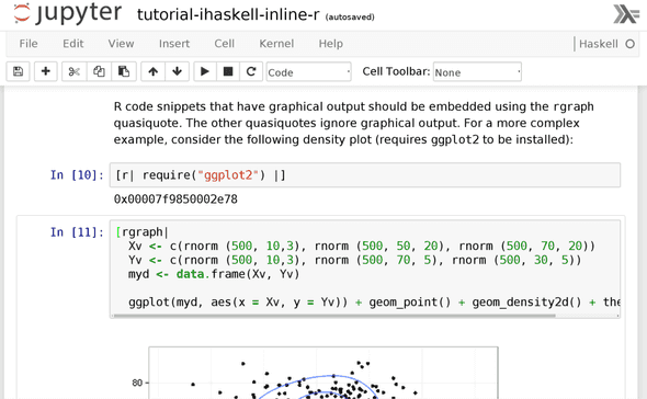
We’ll touch upon each of the above points in more detail below and in future posts. But first, let’s get a taste of this stuff. You may want to consider the below setup as your go-to interactive shell if you haven’t already: it reuses existing projects and works much like GHCi, in an isolated sandbox if you like, except that you have inline graphics and formulas out-of-the-box, as Shae Erisson first pioneered in the Haskell world with ghclive and Manuel Chakravarty realized more recently on OS X with Haskell for Mac.

Charts, code, prose and formulas in a playground

HaskellR features two interactive prompts:

• a bare bones REPL, called H. This is a thin wrapper around GHCi initializing it with all the right extensions and imports to hit the road running;
• an all singing, all dancing interactive notebook, powered by Jupyter (formerly IPython) and Andrew Gibiansky’s fantastic IHaskell kernel.

In this post, we’ll talk mostly about the latter. Thanks to stack, getting started with HaskellR is pretty straightforward, and more importantly, comparatively reliable. We put together a Docker container to get you started hassle-free. It includes Jupyter and IHaskell preinstalled. To build HaskellR inside it:

$ git clone http://github.com/tweag/HaskellR
$ cd HaskellR
$ stack --docker build
$ stack --docker exec ihaskell install

And get started in your browser:

$ stack --docker exec ipython notebook

Or remain in your terminal:

$ stack --docker exec ipython

With IHaskell, you can keep your notes and formulas together with your code in one place, called a notebook. With HaskellR’s plugin for IHaskell, you can use widely acclaimed and very popular R visualization packages such as ggplot2 for embedding plots in your notebook. Working in notebooks (aka playgrounds) is convenient: they are self contained units that is easy to share with colleagues, via email or on the web, and you can edit earlier definitions while keeping the later ones in sync.

Here’s a simple example of using R’s data analysis facilities on data generated in Haskell. Say you have a cluster of noisy data. We’ll use the random package to generate a sample set:

import Control.Monad
import System.Random.MWC as MWC
import System.Random.MWC.Distributions

main = do
  gen <- MWC.create
  xs <- replicateM 500 $ normal 10 3 gen
  ys <- replicateM 500 $ normal 10 3 gen
  ...

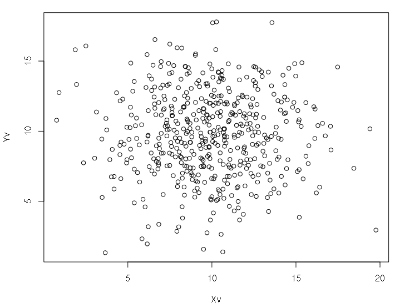
We can now plot the list of x-ordinates against the list of y-ordinates using R’s standard library plot() function:

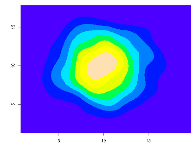
  [r| plot(xs_hs, ys_hs) |]

Better yet: say we want some kind of visualization of the density estimation of these points. We can use R’s 2D kernel density estimation function, available out-of-the-box:

[r| k <- kde2d(Xv, Yv, n=500)
    image(k, col=topo.colors(8)) |]

Notice how in the above, some code appears delineated in quasiquotation blocks. This is a syntactic facility to tell the Haskell compiler that any code inside the block should be understood to be in R’s syntax, not Haskell’s syntax as is normally the case outside of these blocks. We implemented a mechanism to get an embedded instance of the R interpreter to parse that code for us, so that we don’t have to grok R’s full surface syntax ourselves.

By convention, _hs suffixed variables don’t refer to bindings in the R environment, but rather to bindings in the Haskell environment. In technical terms, these variables are actually antiquotations (we use convention over extra syntax so that we can reuse R’s stock parser as-is and not implement our own). Antiquotation is the fundamental mechanism for communicating data between R and Haskell. In common cases, we can do so with no marshalling at all, so you can cross the language boundaries repeatedly in a tight loop with impunity if you like.

Elements of design

The core idea behind HaskellR is that language interop should be zero-cost, or close to. There should be no reason why you would hesitate to dip into a little bit of R to get the job done, over reimplementing the same thing in Haskell because you’re worried about performance or the cost of sending large volumes of data to some remote R interpreter instance. We believe that making foreign calls practically as fast as native calls is the key to making the experience programming with both CRAN and Hackage package functions at the same time seamless.

To this end, we decided to embed the R interpreter instance, that is to say link together in the same binary the C code of the R interpreter with the Haskell code of Haskell programs. In this way, we can communicate with the R interpreter in the same process address space. Many R functions are actually written in C, for speed, and compile down to native code. Some of these primitives can be called from Haskell as cheaply as any other foreign function call.

But that’s not the end of the performance story. A typically vexing issue in cross-language programming is that the one language insists on one representation of the data, while the other language wants its own representation. Therefore, data typically has to be marshalled from one representation to another constantly. In HaskellR, we solved that problem in the following way: just use R’s representation throughout. It’s the form that R functions expect, so they can get straight to computing on that data when called. The trouble is, R’s data representation is foreign to Haskell, so you lose Haskell’s extremely powerful language facilities that work with any native algebraic datatype, such as pattern matching. Or do you?…

The trick to get the best of both worlds, zero marshalling but also pattern matching, is to define so-called view functions that provide you with a native view as an algebraic datatype of the foreign data. Here’s a toy and contrived example, where we define the factorial function in Haskell but over R integers:

fact :: SEXP s 'R.Int -> R s (SEXP s 'R.Int)
fact (hexp -> Int [0]) = R.cast sing <$> [r| 1L |]
fact n@(hexp -> Int _) =
    R.cast sing <$> [r| n_hs * fact_hs(n_hs - 1L) |]

hexp is a view function, mapping native R data (everything is a SEXP internally in R) to a Haskell-native GADT. Thanks to the type annotations (more on that in future posts), we know statically that the R data can only be some kind of integer vector, so we pattern match on that, check whether it’s the singleton zero vector or not, and recurse.

Aren’t we now back to marshalling? Yes and no! We carefully engineered these view functions to be non-recursive. Non-recursive functions can be inlined. So that when you use a view function only to pattern match on the result immediately afterwards, as is the case above, GHC is smart enough to recognize that the view function is constructing a datatype value only to destructure it later, so it simplifies the allocation away! Yes this is marshalling of sorts, but it’s marshalling for free: there is no trace of it at runtime.

There’s plenty more to talk about regarding the design of HaskellR, but this post is already getting long, so we’ll keep a few topics for next time.

Future work

In the meantime, there’s plenty more to work on, so feel free to jump in and contribute to the project. In the end what HaskellR provides is a way to write Haskell programs piecing together R primitives at native speed rather than doing so via semi-structured R scripts. But we haven’t entirely removed the overhead of calling these R primitives just yet. The next steps:

• direct access to primitives written in C without incurring at runtime the cost of a lookup due to R’s dynamic binding. Currently, this involves poking a bit deeper into the internals of R than is entirely reasonable, but we’re working to make this easier in future versions of R.
• Better Windows support: currently Windows support is highly experimental, and the installation instructions need to be sorted out. Any help appreciated.
• Alexander Vershilov has contributed a new implementation of quasiquoters that should significantly speed up compile times for large quasiquotations.

If you’re interested in this line of work and want to keep abreast of any significant updates, do sign up to the HaskellR mailing list.

Special thanks to Dave Balaban for his help and support, and to the early users of HaskellR and previous incarnations.