Introduction
Haskell and data science - on first sight a great match: native function composition, lazy evaluation, fast execution times, and lots of code checks. These sound like ingredients for scalable, production-ready data transformation pipelines. What is missing then? Why is Haskell not widely used in data science?
One of the reasons is that Haskell lacks a standardized data analysis
environment. For example, Python has a de facto standard library set with
numpy, pandas and scikit-learn that form the backbone, and many other
well-supported specialized libraries such as keras and tensorflow that are
easily accessible. These libraries are distributed with user friendly package
managers and explained in a plethora of tutorials, Stack Overflow questions and
millions of Jupyter notebooks. Most problems from beginner to advanced level
can be solved by adapting and combining these existing solutions.
This post presents Jupyter and JupyterLab - both important ingredients of the Python ecosystem - and shows how we can take advantage of these tools for interactive data analysis in Haskell.
Jupyter and exploratory data analysis
Project Jupyter became famous through the browser-based notebook app that allows to execute code in various compute environments and interlace it with text and media elements (example gallery).
More generally, Project Jupyter standardizes the interactions between Jupyter frontends such as the notebook and Jupyter kernels, the compute environments. Typically a kernel receives a message from a frontend, executes some code, and responds with a rich media message. The frontend can render the response message as text, images, videos or small applications. All exchanged messages are standardized by the Jupyter protocol and therefore independent of the specific frontend or kernel that is used. Various frontends and kernels for many different languages, like Python, Haskell, R, C++, Julia, etc, exist.
Quick REPL-like interaction of a user with a compute environment via a frontend is very useful for exploratory data analysis. The user interrogates and transforms the data with little code snippets and receives immediate feedback through rich media responses. Different algorithms (expressed as short code snippets) can rapidly be prototyped and visualized. Long multistep dialogues with the kernel can be assembled into a sequential notebook. Notebooks mix explanatory text, code and media elements and can therefore be used as human-readable reports (such as this blogpost). This REPL workflow has become one of the most popular ways for exploratory data analysis.
Conversations with a Jupyter kernel
IHaskell is the name of the Jupyter
kernel for Haskell. It contains a little executable ihaskell that can receive
and respond to messages in the Jupyter protocol (via
ZeroMQ. Here is a little dialogue that is
initiated by sending the following code snippet from the notebook frontend to
ihaskell:
take 10 $ (^2) <$> [1..]And here is the rendered answer that the frontend received from the kernel
[1,4,9,16,25,36,49,64,81,100]
In Jupyter parlance the above dialogue corresponds to the following
execute_request:
>> shell.execute_request (8be63d5c-1170-495d-82da-e56272052faf) <<

header: {username: "", version: "5.2",
         session: "32fe9cd0-8c37-450e-93c0-6fbd45bfdcd9",
         msg_id: "8be63d5c-1170-495d-82da-e56272052faf",
         msg_type: "execute_request"}
parent_header: Object
channel: "shell"
content: {silent: false, store_history: true, user_expressions: Object,
          allow_stdin: true, stop_on_error: true,
          code: "take 10 $ (^2) <$> [1..]"}   <<<<< LOOK HERE
metadata: Object
buffers: Array[0]
and to the following display_data message that is received as a response
<< iopub.display_data (68cce1e7-4d60-4a20-a707-4bf352c4d8d2) >>

header: {username: "", msg_type: "display_data", version: "5.0"
         msg_id: "68cce1e7-4d60-4a20-a707-4bf352c4d8d2",
         session: "32fe9cd0-8c37-450e-93c0-6fbd45bfdcd9",
         date: "2018-08-02T08:14:10.245877Z"}
msg_id: "68cce1e7-4d60-4a20-a707-4bf352c4d8d2"
msg_type: "display_data"
parent_header: {username: "", msg_type: "execute_request", version: "5.0",
                msg_id: "8be63d5c-1170-495d-82da-e56272052faf",
                session: "32fe9cd0-8c37-450e-93c0-6fbd45bfdcd9"}
metadata: Object
content: {data: {text/plain: "[1,4,9,16,25,36,49,64,81,100]"},  <<<<< LOOK HERE
          metadata: {output_type: "display_data"}}
buffers: Array[0]
channel: "iopub"
ihaskell can import Haskell libraries dynamically and has some special
commands to enable language extensions, print type information or to use
Hoogle.
JupyterLab
JupyterLab is the newest animal in the Jupyter frontend zoo, and it is arguably the most powerful: console, notebook, terminal, text-editor, or image viewer, JupyterLab integrates these data science building blocks into a single web based user interface. JupyterLab is setup as a modular system that can be extended. A module assembles the base elements, changes or add new features to build an IDE, a classical notebook or even a GUI where all interactions with the underlying execution kernels are hidden behind graphical elements.
How can Haskell take advantage of JupyterLab’s capacities? To begin with,
JupyterLab provides plenty of out-of-the-box renderers that can be used for
free by Haskell. From the default
renderers,
the most interesting is probably Vega plotting. But also geojson, plotly or
and many other formats are available from the list of extensions, which will
certainly grow. Another use case might be to using the JupyterLab extension
system makes it easy to build a simple UI that interact with an execution
environment. Finally, Jupyter and associated workflows are known by a large
community. Using Haskell through these familiar environments softens the
barrier that many encounter when exploring Haskell for serious data science.
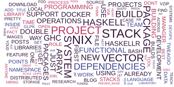
Let’s get into a small example that shows how to use the JupyterLab VEGA renderer with IHaskell.
Wordclouds using Haskell, Vega and JupyterLab
We will use here the word content of all blog posts of tweag.io, which are
written in markdown text files. The following little code cell that reads all
.md files in the posts folder and concatenates them into a single long
string from which we remove some punctuation characters. This code cell is then
sent to the ihaskell kernel, which responds to the last take function with
a simple text response.
:ext QuasiQuotes
import System.Directory
import Data.List

fnames <- getDirectoryContents "../../posts"
paths = ("../../posts/"++) <$> fnames
md_files = filter (isSuffixOf ".md") paths
text <- mconcat (readFile <$> md_files)
cleanedText = filter (not . (`elem` "\n,.?!-:;\"\'")) text
take 50 cleanedText
"title Were hiring<br>(Software engineer / devops)p"The VEGA visualization specification for a wordcloud can be defined as a JSON
string that is filled with our text data. A convenient way to write longer
multiline strings in Haskell are QuasiQuotes. We use fString QuasiQuotes
from the PyF package.
Note that {} fills in template data and {{ corresponds to an escaped {.
import Formatting
import PyF
import Data.String.QQ

let vegaString = [fString|{{
  "$schema": "https://vega.github.io/schema/vega/v4.json",
  "width": 800,
  "height": 400,
  "padding": 0,

  "data": [
    {{
      "name": "table",
      "values": [
         "{take 20000 cleanedText}"
      ],
      "transform": [
        {{
          "type": "countpattern",
          "field": "data",
          "case": "upper",
          "pattern": "[\\\\w']{{3,}}",
          "stopwords": "(\\\\d+|youll|looking|like|youre|etc|yet|need|cant|ALSO|STILL|ISNT|Want|Lots|HTTP|HTTPS|i|me|my|myself|we|us|our|ours|ourselves|you|your|yours|yourself|yourselves|he|him|his|himself|she|her|hers|herself|it|its|itself|they|them|their|theirs|themselves|what|which|who|whom|whose|this|that|these|those|am|is|are|was|were|be|been|being|have|has|had|having|do|does|did|doing|will|would|should|can|could|ought|i'm|you're|he's|she's|it's|we're|they're|i've|you've|we've|they've|i'd|you'd|he'd|she'd|we'd|they'd|i'll|you'll|he'll|she'll|we'll|they'll|isn't|aren't|wasn't|weren't|hasn't|haven't|hadn't|doesn't|don't|didn't|won't|wouldn't|shan't|shouldn't|can't|cannot|couldn't|mustn't|let's|that's|who's|what's|here's|there's|when's|where's|why's|how's|a|an|the|and|but|if|or|because|as|until|while|of|at|by|for|with|about|against|between|into|through|during|before|after|above|below|to|from|up|upon|down|in|out|on|off|over|under|again|further|then|once|here|there|when|where|why|how|all|any|both|each|few|more|most|other|some|such|no|nor|not|only|own|same|so|than|too|very|say|says|said|shall)"
        }},
        {{
          "type": "formula", "as": "angle",
          "expr": "[0, 90][~~(random() * 3)]"
        }},
        {{
          "type": "formula", "as": "weight",
          "expr": "if(datum.text=='VEGA', 600, 300)"
        }}
      ]
    }}
  ],

  "scales": [
    {{
      "name": "color",
      "type": "ordinal",
      "range": ["#3e4593", "#bc3761", "#39163d", "#2a1337"]
    }}
  ],

  "marks": [
    {{
      "type": "text",
      "from": {{"data": "table"}},
      "encode": {{
        "enter": {{
          "text": {{"field": "text"}},
          "align": {{"value": "center"}},
          "baseline": {{"value": "alphabetic"}},
          "fill": {{"scale": "color", "field": "text"}}
        }},
        "update": {{
          "fillOpacity": {{"value": 1}}
        }},
        "hover": {{
          "fillOpacity": {{"value": 0.5}}
        }}
      }},
      "transform": [
        {{
          "type": "wordcloud",
          "size": [800, 400],
          "text": {{"field": "text"}},
          "rotate": {{"field": "datum.angle"}},
          "font": "Helvetica Neue, Arial",
          "fontSize": {{"field": "datum.count"}},
          "fontWeight": {{"field": "datum.weight"}},
          "fontSizeRange": [12, 56],
          "padding": 2
        }}
      ]
    }}
  ]
}}|]
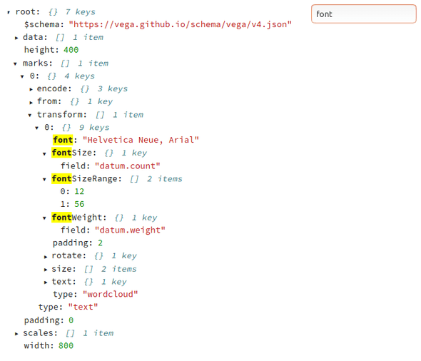
We display this JSON string with the native Jupyterlab JSON renderer here for
convenience. The Display.json function from IHaskell annotates the content of
the display message as application/json and ihaskell sends the annotated
display message to Jupyterlab. In consequence, Jupyterlab knows that it should
use its internal application/json renderer to display the message in the
frontend.
import qualified IHaskell.Display as D
D.Display [D.json vegaString]
In a similar way, we can annotate the display message with the
application/vnd.vegalite.v2+json MIME renderer type. The VEGA string that we
have generated earlier is then rendered with the internal JupyterLab javascript
VEGA code:
D.Display [D.vegalite vegaString]Conclusion
JupyterLab provides a REPL-like workflow that is convenient for quick exploratory data analysis and reporting. Haskell can benefit in particular from JupyterLab’s rendering capacities, its pleasant user interface and its familiarity in the data science community. If you want to try it yourself, this blog post has been written directly as a notebook that is stored in this folder (with a dataset from Wikipedia). The IHaskell setup with this example notebook is available as a docker image that you can run with:
docker run -p 8888:8888 tweag/jupyterwith:latestAlternatively, if you are a Nix user, you can try our declarative JupyterLab-on-Nix setup that is the subject of our next post.
Behind the scenes
Matthias is a scientist and developer who worked at Tweag. He says he's a generalist "half scientist, half musician, and a third half of other things" but you'll have to ask him what that means exactly! He lives in Paris, and enjoys a good discussion, writing long-form texts in vim or reading and occasionally writing code.
If you enjoyed this article, you might be interested in joining the Tweag team.

