This is part 2 of a series of blog posts about MCMC techniques:
- Part I: The basics and Metropolis-Hastings
- Part III: Hamiltonian Monte Carlo
- Part IV: Replica Exchange
In the first blog post of this series, we discussed Markov chains and the most elementary MCMC method, the Metropolis-Hastings algorithm, and used it to sample from a univariate distribution. In this episode, we discuss another famous sampling algorithm: the (systematic scan) Gibbs sampler. It is very useful to sample from multivariate distributions: it reduces the complex problem of sampling from a joint distribution to sampling from the full conditional (meaning, conditioned on all other variables) distribution of each variable. That means that to sample from, say, p(x,y), it is sufficient to be able to sample from p(x∣y) and p(y∣x), which might be considerably easier. The problem of sampling from multivariate distributions often arises in Bayesian statistics, where inference of likely values for a parameter often entails sampling not only that parameter, but also additional parameters required by the statistical model.
Motivation
Why would splitting up sampling in this way be preferable? Well, it might turn the problem of sampling from one untractable joint distribution into sampling from several well-known, tractable distributions. If the latter (now conditional) distributions are still not tractable, at least you now can use different and well-suited samplers for each of them instead of sampling all variables with a one-size-fits-all sampler. Take, for example, a bivariate normal distribution with density p(x,y) that has very different variances for each variable:
import numpy as np

def log_gaussian(x, mu, sigma):
    # The np.sum() is for compatibility with sample_MH
    return - 0.5 * np.sum((x - mu) ** 2) / sigma ** 2 \
           - np.log(np.sqrt(2 * np.pi * sigma ** 2))


class BivariateNormal(object):
    n_variates = 2

    def __init__(self, mu1, mu2, sigma1, sigma2):
        self.mu1, self.mu2 = mu1, mu2
        self.sigma1, self.sigma2 = sigma1, sigma2

    def log_p_x(self, x):
        return log_gaussian(x, self.mu1, self.sigma1)

    def log_p_y(self, x):
        return log_gaussian(x, self.mu2, self.sigma2)

    def log_prob(self, x):
        cov_matrix = np.array([[self.sigma1 ** 2, 0],
                               [0, self.sigma2 ** 2]])
        inv_cov_matrix = np.linalg.inv(cov_matrix)
        kernel = -0.5 * (x - self.mu1) @ inv_cov_matrix @ (x - self.mu2).T
        normalization = np.log(np.sqrt((2 * np.pi) ** self.n_variates * np.linalg.det(cov_matrix)))

        return kernel - normalization


bivariate_normal = BivariateNormal(mu1=0.0, mu2=0.0, sigma1=1.0, sigma2=0.15)
The @ is a recent-ish addition to Python and denotes the matrix multiplication operator.
Let’s plot this density:
Now you can try to sample from this using the previously discussed Metropolis-Hastings algorithm with a uniform proposal distribution. Remember that in Metropolis-Hastings, a Markov chain is built by jumping a certain distance (“step size”) away from the current state, and accepting or rejecting the new state according to an acceptance probability. A small step size will explore the possible values for x very slowly, while a large step size will have very poor acceptance rates for y. The Gibbs sampler allows us to use separate Metropolis-Hastings samplers for x and y - each with an appropriate step size. Note that we could also choose a bivariate proposal distribution in the Metropolis-Hastings algorithm such that its variance in x-direction is larger than its variance in the y-direction, but let’s stick to this example for didactic purposes.
The systematic scan Gibbs sampler
So how does Gibbs sampling work? The basic idea is that given the joint distribution p(x,y) and a state (xi,yi) from that distribution, you obtain a new state as follows: first, you sample a new value for one variable, say, xi+1, from its distribution conditioned on yi, that is, from p(x∣yi). Then, you sample a new state for the second variable, yi+1, from its distribution conditioned on the previously drawn state for x, that is, from p(y∣x_i+1). This two-step procedure can be summarized as follows:
This is then iterated to build up the Markov chain. For more than two variables, the procedure is analogous: you pick a fixed ordering and draw one variable after the other, each conditioned on, in general, a mix of old and new values for all other variables.1 Fixing an ordering, like this, is called a systematic scan, an alternative is the random scan where we’d randomly pick a new ordering at each iteration.
Implementing this Gibbs sampler for the above example is extremely simple, because the two variables are independent (p(x∣y)=p(x) and p(y∣x)=p(y)).
We sample each of them with a Metropolis-Hastings sampler, implemented in the first blog post as the sample_MH function.
As a reminder, that function takes as arguments, in that order,
- the old state of a Markov chain (a one-dimensional
numpyarray), - a function returning the logarithm of the probability density function (PDF) to sample from,
- a real number representing the step size for the uniform proposal distribution, from which a new state is proposed.
We then use sample_MH in the following, short function which implements the systematic scan Gibbs sampler:
def sample_gibbs(old_state, bivariate_dist, stepsizes):
    """Draws a single sample using the systematic Gibbs sampling
    transition kernel

    Arguments:
    - old_state: the old (two-dimensional) state of a Markov chain
                 (a list containing two floats)
    - bivariate_dist: an object representing a bivariate distribution
                      (in our case, an instance of BivariateNormal)
    - stepsizes: a list of step sizes

    """
    x_old, y_old = old_state

    # for compatibility with sample_MH, change floats to one-dimensional
    # numpy arrays of length one
    x_old = np.array([x_old])
    y_old = np.array([y_old])

    # draw new x conditioned on y
    p_x_y = bivariate_dist.log_p_x
    accept_x, x_new = sample_MH(x_old, p_x_y, stepsizes[0])

    # draw new y conditioned on x
    p_y_x = bivariate_dist.log_p_y
    accept_y, y_new = sample_MH(y_old, p_y_x, stepsizes[1])

    # Don't forget to turn the one-dimensional numpy arrays x_new, y_new
    # of length one back into floats

    return (accept_x, accept_y), (x_new[0], y_new[0])
The sample_gibbs function will yield one single sample from bivariate_normal.
As we did in the previous blog post for the Metropolis-Hastings algorithm, we now write a function that repeatedly runs sample_gibbs to build up a Markov chain and call it:
def build_gibbs_chain(init, stepsizes, n_total, bivariate_dist):
    """Builds a Markov chain by performing repeated transitions using
    the systematic Gibbs sampling transition kernel

    Arguments:
    - init: an initial (two-dimensional) state for the Markov chain
            (a list containing two floats)
    - stepsizes: a list of step sizes of type float
    - n_total: the total length of the Markov chain
    - bivariate_dist: an object representing a bivariate distribution
                      (in our case, an instance of BivariateNormal)

    """
    init_x, init_k = init
    chain = [init]
    acceptances = []

    for _ in range(n_total):
        accept, new_state = sample_gibbs(chain[-1], bivariate_dist, stepsizes)
        chain.append(new_state)
        acceptances.append(accept)

    acceptance_rates = np.mean(acceptances, 0)
    print("Acceptance rates: x: {:.3f}, y: {:.3f}".format(acceptance_rates[0],
                                                          acceptance_rates[1]))

    return chain

stepsizes = (6.5, 1.0)
initial_state = [2.0, -1.0]
chain = build_gibbs_chain(initial_state, stepsizes, 100000, bivariate_normal)
chain = np.array(chain)
Acceptance rates: x: 0.462, y: 0.456Tada!
We used two very different step sizes and achieved very similar acceptance rates with both.
We now plot a 2D histogram of the samples (with the estimated probability density color-coded) and the marginal distributions:
plot_bivariate_samples(chain, burnin=200, pdf=bivariate_normal)Looking at the path the Markov chain takes, we see several horizontal and vertical lines. These are Gibbs sampling steps in which only one of the Metropolis-Hastings moves was accepted.
A more complex example
The previous example was rather trivial in the sense that both variables were independent. Let’s discuss a more interesting example, which features both a discrete and a continuous variable. We consider a mixture of two normal densities p_N(x;μ,σ) with relative weights w1 and w2. The PDF we want to sample from is then
This probability density is just a weighted sum of normal densities. Let’s consider a concrete example, choosing the following mixture parameters:
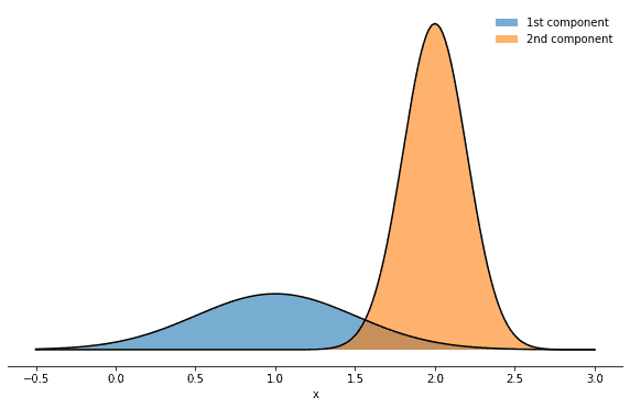
mix_params = dict(mu1=1.0, mu2=2.0, sigma1=0.5, sigma2=0.2, w1=0.3, w2=0.7)How does it look like? Well, it’s a superposition of two normal distributions:
Inspired by this figure, we can also make the mixture nature of that density more explicit by introducing an additional integer variable k∈1,2 which enumerates the mixture components. This will allow us to highlight several features and properties of the Gibbs sampler and to introduce an important term in probability theory along the way. Having introduced a second variable means that we can consider several probability distributions:
- p(x,k): the joint distribution of x and k tells us how probable it is to find a value for x and a value for k “at the same time” and is given by
- p(x∣k): the conditional distribution of x given k tells us the probability of x for a certain k. For example, if k=1, what is p(x∣k)? Setting k=1 means we’re considering only the first mixture component, which is a normal distribution with mean μ1 and standard deviation σ1 and thus p(x∣k=1)=pN(x;μ1,σ1). In general we then have
- p(k∣x): assuming a certain value x, this probability distribution tells us for each k the probability with which you would draw x from the mixture component with index k. This probability is non-trivial, as the mixture components overlap and each x thus has a non-zero probability in each component. But Bayes’ theorem saves us and yields
- p(k): this is the probability of choosing a mixture component k irrespective of x and is given by the mixture weights wk.
The probability distributions p(x) and p(k) are related to the joint distribution p(x,k) by a procedure called marginalization. We marginalize p(x,k) over, say, k, when we are only interested in the probability of x, independent of a specific value for k. That means that the probability of x is the sum of the probability of x when k=1 plus the probability of x when k=2, or, formally,
With these probability distributions, we have all the required ingredients for setting up a Gibbs sampler. We can then sample from p(x,k) and reconstruct p(x) by marginalization. As marginalization means “not looking a variable”, obtaining samples from p(x) given samples from p(x,k) just amounts to discarding the sampled values for k.
Let’s first implement a Gaussian mixture with these conditional distributions:
class GaussianMixture(object):

    def __init__(self, mu1, mu2, sigma1, sigma2, w1, w2):
        self.mu1, self.mu2 = mu1, mu2
        self.sigma1, self.sigma2 = sigma1, sigma2
        self.w1, self.w2 = w1, w2

    def log_prob(self, x):
        return np.logaddexp(np.log(self.w1) + log_gaussian(x, self.mu1, self.sigma1),
                            np.log(self.w2) + log_gaussian(x, self.mu2, self.sigma2))

    def log_p_x_k(self, x, k):
        # logarithm of p(x|k)
        mu = (self.mu1, self.mu2)[k]
        sigma = (self.sigma1, self.sigma2)[k]

        return log_gaussian(x, mu, sigma)

    def p_k_x(self, k, x):
        # p(k|x) using Bayes' theorem
        mu = (self.mu1, self.mu2)[k]
        sigma = (self.sigma1, self.sigma2)[k]
        weight = (self.w1, self.w2)[k]
        log_normalization = self.log_prob(x)

        return np.exp(log_gaussian(x, mu, sigma) + np.log(weight) - log_normalization)
The interesting point here (and, in fact, the reason I chose this example) is that p(x∣k) is a probability density for a continuous variable x, while p(k∣x) is a probability distribution for a discrete variable. This means we will have to choose two very different sampling methods.
While we could just use a built-in numpy function to draw from the normal distributions p(x∣k), we will use Metropolis-Hastings.
The freedom to do this really demonstrates the flexibility we have in choosing samplers for the conditional distributions.
So we need to reimplement sample_gibbs and build_gibbs_chain, whose arguments are very similar to the previous implementation, but with a slight difference: the states now consist of a float for the continuous variable and an integer for the mixture component, and instead of a list of stepsizes we just need one single stepsize, as we have only one variable to be sampled with Metropolis-Hastings.
def sample_gibbs(old_state, mixture, stepsize):
    """Draws a single sample using the systematic Gibbs sampling
    transition kernel

    Arguments:
    - old_state: the old (two-dimensional) state of a Markov chain
                 (a list containing a float and an integer representing
                 the initial mixture component)
    - mixture: an object representing a mixture of densities
               (in our case, an instance of GaussianMixture)
    - stepsize: a step size of type float

    """
    x_old, k_old = old_state

    # for compatibility with sample_MH, change floats to one-dimensional
    # numpy arrays of length one
    x_old = np.array([x_old])

    # draw new x conditioned on k
    x_pdf = lambda x: mixture.log_p_x_k(x, k_old)
    accept, x_new = sample_MH(x_old, x_pdf, stepsize)

    # ... turn the one-dimensional numpy arrays of length one back
    # into floats
    x_new = x_new[0]

    # draw new k conditioned on x
    k_probabilities = (mixture.p_k_x(0, x_new), mixture.p_k_x(1, x_new))
    jump_probability = k_probabilities[1 - k_old]
    k_new = np.random.choice((0,1), p=k_probabilities)

    return accept, jump_probability, (x_new, k_new)


def build_gibbs_chain(init, stepsize, n_total, mixture):
    """Builds a Markov chain by performing repeated transitions using
    the systematic Gibbs sampling transition kernel

    Arguments:
    - init: an initial (two-dimensional) state of a Markov chain
            (a list containing a one-dimensional numpy array
            of length one and an integer representing the initial
            mixture component)
    - stepsize: a step size of type float
    - n_total: the total length of the Markov chain
    - mixture: an object representing a mixture of densities
               (in our case, an instance of GaussianMixture)

    """
    init_x, init_k = init
    chain = [init]
    acceptances = []
    jump_probabilities = []

    for _ in range(n_total):
        accept, jump_probability, new_state = sample_gibbs(chain[-1], mixture, stepsize)
        chain.append(new_state)
        jump_probabilities.append(jump_probability)
        acceptances.append(accept)

    acceptance_rates = np.mean(acceptances)
    print("Acceptance rate: x: {:.3f}".format(acceptance_rates))
    print("Average probability to change mode: {}".format(np.mean(jump_probabilities)))

    return chain

mixture = GaussianMixture(**mix_params)
stepsize = 1.0
initial_state = [2.0, 1]
chain = build_gibbs_chain(initial_state, stepsize, 10000, mixture)
burnin = 1000
x_states = [state[0] for state in chain[burnin:]]
Acceptance rate: x: 0.631
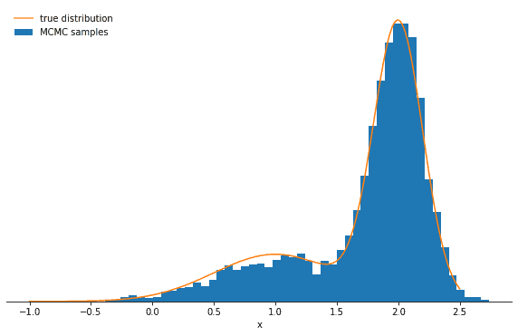
Average probability to change mode: 0.08629295966662387Plotting a histogram of our samples shows that the Gibbs sampler correctly reproduces the desired Gaussian mixture:
You might wonder why we’re also printing the average probability for the chain to sample from the component it is currently not in. If this probability is very low, the Markov chain will get stuck for some time in the current mode and thus will have difficulties exploring the distribution rapidly. The quantity of interest here is p(k∣x): it is the probability of a certain component k given a certain value x and can be very low if the components are more separated and x is more likely to be in the component which is not k. Let’s explore this behavior by increasing the separation between the means of the mixture components:
mixture = GaussianMixture(mu1=-1.0, mu2=2.0, sigma1=0.5, sigma2=0.2, w1=0.3, w2=0.7)
stepsize = 1.0
initial_state = [2.0, 1]
chain = build_gibbs_chain(initial_state, stepsize, 100000, mixture)
burnin = 10000
x_states = [state[0] for state in chain[burnin:]]
Acceptance rate: x: 0.558
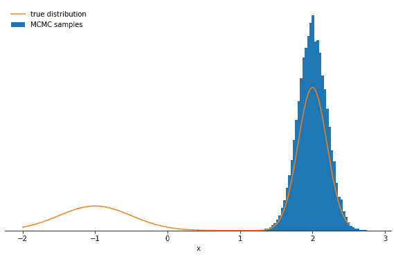
Average probability to change mode: 6.139534006013391e-06Let’s plot the samples and the true distribution and see how the Gibbs sampler performs in this case:
You should see the probability decrease significantly and perhaps one of the modes being strongly over- and the other undersampled. The lesson here is that the Gibbs sampler might produce highly correlated samples. Again—in the limit of many, many samples—the Gibbs sampler will reproduce the correct distribution, but you might have to wait a long time.
Conclusions
By now, I hope you have a basic understanding of why Gibbs sampling is an important MCMC technique, how it works, and why it can produce highly correlated samples.
I encourage you again to download the full notebook and play around with the code:
you could try using the normal function from the numpy.random module instead of Metropolis-Hastings in both examples or implement a random scan, in which the order in which you sample from the conditional distributions is chosen randomly.
Or you could read about and implement the collapsed Gibbs sampler, which allows you to perfectly sample the Gaussian mixture example by sampling from p(k) instead of p(k∣x). Or you can just wait a little more for the next post in the series, which will be about Hybrid Monte Carlo (HMC), a fancy Metropolis-Hastings variant which takes into account the derivative of the log-probability of interest to propose better, less correlated, states!
- It’s important to note, though, that the transition kernel given by the above procedure does not define a detailed-balanced transition kernel for a Markov chain on the joint space of x and y. One can show, though, that for each single variable, this procedure is a detailed-balanced transition kernel and the Gibbs sampler thus constitutes a composition of Metropolis-Hastings steps with acceptance probability 1. For details, see, for example, this stats.stackexchange.com answer.↩
Behind the scenes
Simeon is a theoretical physicist who has undergone several transformations. A journey through Markov chain Monte Carlo methods, computational structural biology, a wet lab and renowned research institutions in Germany, Paris and New York finally led him back to Paris and to Tweag, where he is currently leading projects for a major pharma company. During pre-meeting smalltalk, ask him about rock climbing, Argentinian tango or playing the piano!
If you enjoyed this article, you might be interested in joining the Tweag team.


